Iterative samplers
Here's some illustrations of the theorem that a stationary sampler converges iff the corresponding stationary linear solver converges
(Fox & Parker, Bernoulli, 2016; Fox & Parker, SISC, 2014).
Here's an image of Gibbs iterates from a 2-D dimensional Gaussian in the typical coordinate
directions. 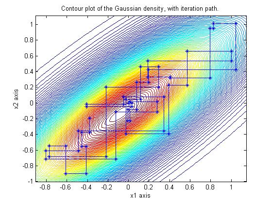
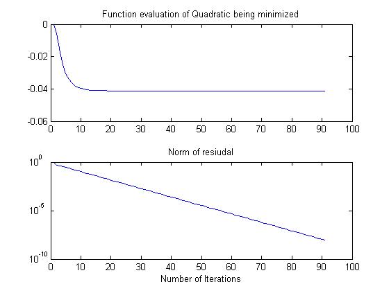
The Gauss-Siedel iteration which minimizes the corresponding quadratic using the same
coordinate directions converges geometrically (i.e., linear on the log scale) in 90
iterations: 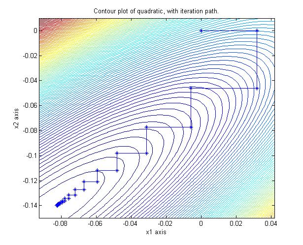
When accelerated with Chebyshev polynomials, the sampling directions are more in line
with the eigen-directions of maximal variability. 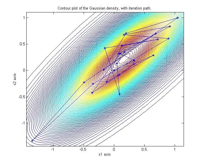
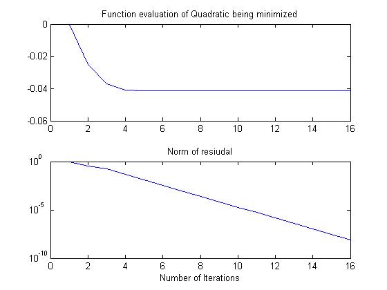
The Chebyshev accelerated forward-backward sweeps of Gauss-Siedel on the corresponding
quadratic converges in 15 iterations: 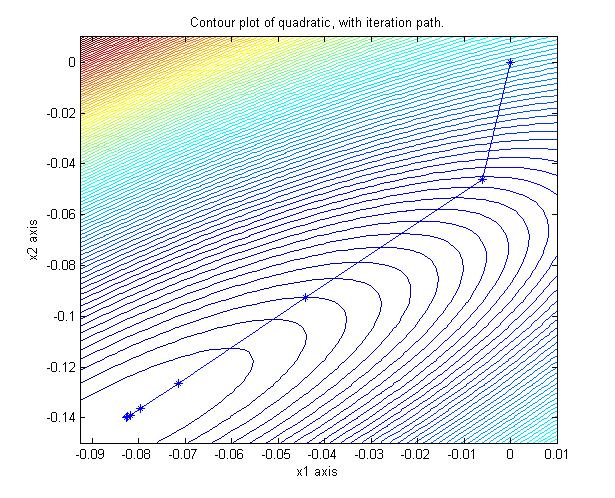
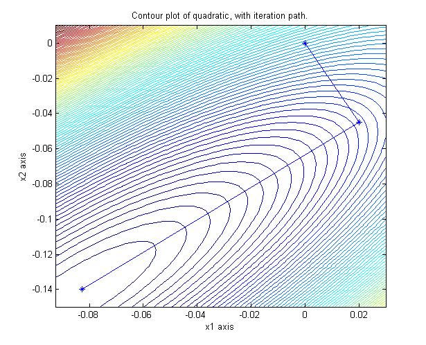
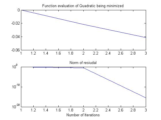
Acceleration by non-stationary Conjugate Gradients (or Lanczos vectors) works in theory,
but implementation in finite precision is a work in progress (Parker & Fox, SISC, 2012; Parker et al., JASA, 2016). As expected from results from numerical linear algebra, a CG (or CD) sampler's
performance depends on the distribution of the eigenvalues of the covariance matrix.
2-D is easy to sample from, shown here are iterates from a Lanczos implementation
of a CG accelerated Gibbs sampler: 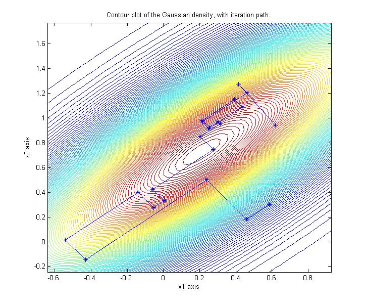
Unlike other iterative linear solvers, a CG linear solve finds the minimum of the
corresponding quadratic in a finite number of iterations (ie faster than geometric
convergence):